Advanced R for Econometricians
Advanced R Concepts
Martin C. Arnold, Jens Klenke
Overview
Make sure the lobstr package is attached!
install.packages('lobstr')library(lobstr)Outline
Names and values
Bindings and references
Copy-on-modify / in-place modification
Unbinding and Garbage Collection
Functions
Fundamentals, scoping and Lazy Evaluation
Function forms
Names and Values
Assignment Operators
<-is often used for assignment but some people use=instead.There is, however, a subtle difference in how they are evaluated when mixed in the same expression.
Example: operator precedence
a <- b <- 1a == b## [1] TRUEa = b = 1a == b## [1] TRUEa = b <- 1a == b## [1] TRUEa <- b = 1## Error in a <- b = 1: could not find function "<-<-"This really is just a convention and nothing precludes using
=instead of<-for assignmentWhen mixed,
<-has precedence over=Fact:
<-comes from a time where there actually was a<-key on keyboards.<-and->essentially do the same thing.R interprets
a <- b = 1as'<-<-'(a, b = 1, value = 1)
Assignment Operators
For consistency we use
<-for binding and=for assigning objects to function arguments.Note, however, that there are reasonable proposals for using other conventions.
Task:
Find out what -> does and think of an application where it might be useful.
Hint: Experiment to find out about the precedence relation between <-, -> and =.
->is the right-assignment operatorThe precedence relation is
->>><->>=sox <- 1 -> bis another working alternative to the last line on the previous slide.
Assignment Operators
Assignment operators work in the environment they are invoked in. The super assignment operator <<- assigns in the enclosing environment, provided the binding exists there.
Example: super assignment
var_GE <- 1a <- function(x) { b <- function(x) var_GE <<- x b(x)}a(3)var_GE## [1] 3Note that functions generate their own environments upon execution. The execution environment of
a()is the parent environment tob().If
<<-does not find a corresponding binding in the enclosing environment, it looks in the parent environment and works it's way up towards to global environment (GE)If the binding does not exist in the GE, it will be created there
Bindings
Knowing what assignment does internally is crucial for understanding performance and memory usage of your code and R's functional programming tools.
What happens if we define a vector
x? The idiom 'the objectxstores the vector' is not quite right...
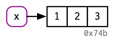
Example: binding a vector
Binding means that the name has a value: x is a reference to a value living in the computer's memory.


Source: Wickham (2019)
x <- c(1, 2, 3)
y <- xBindings — Character Vectors
A character vector is a binding to a vector of strings.
Example: binding a character vector


Source: Wickham (2019)
x <- c("a", "a", "abc", "d")ref(x, character = TRUE)## █ [1:0x10900f248] <chr> ## ├─[2:0x12b2ced78] <string: "a"> ## ├─[2:0x12b2ced78] ## ├─[3:0x10495fc88] <string: "abc"> ## └─[4:0x12b505670] <string: "d">Copy-on-modify
R's copy-on-modify behavior is both blessing and curse:
We may use references without the risk of breaking existing code (convenient).
modifying a reference may trigger a copy of the value (unfavourable).
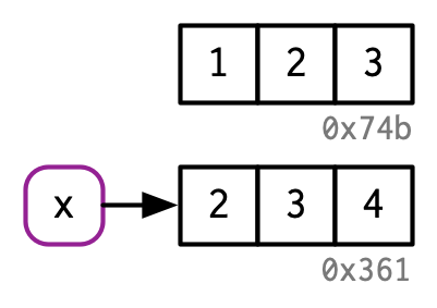
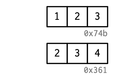
Example: copy-on-modify

Source: Wickham (2019)
x <- c(1, 2, 3)y <- xy[[3]] <- 4x## [1] 1 2 3obj_addr(x)## [1] "0x10900fbf8"obj_addr(y)## [1] "0x109a51258"This is very different for many other languages, including c++ which we will see later during the course.
Question: object addresses (like
0x7f9ef3059d38) will be different (unpredictable) if the code is re-run. Why?
Copy-on-modify
We may use tracemem() to obtain info when a copy of an object is generated.
Example: keeping track of copies using tracemem()
tracemem() returns the copied object, the new address (and the call stack, if functions are involved).
x <- c(1, 2, 3)tracemem(x)[1] "<0x7fba7740ebb8>"
y <- xy[[3]] <- 4tracemem[0x7fba7740ebb8 -> 0x7fba76883958]:
y[[3]] <- 5# stop trackinguntracemem(x)Simply put, a call stack describes the order of nested function calls.
Copy-on-modify — Function Calls
The above rules apply to function calls as well.
Example: keeping track of copies using tracemem() — ctd.

Source: Wickham (2019)
f <- function(a) ax <- c(1, 2, 3)tracemem(x)## [1] "<0x74b050b21318>"z <- f(x) # no copy here!untracemem(x)No copy because z is just a reference to the value of x.
Copy-on-modify — Function Calls
Task:
Predict what tracemem() returns if the highlighted lines get executed, respectively.
f <- function(a) { a[[1]] <- 0 a}x <- c(1, 2, 3)tracemem(x)f(x)z <- f(x)untracemem(x)f(x):f()bindsato the same memory locationxpoints to during execution. In Contrast to the previous slide, a copy is made sincef()modifiesa.z<-f(x): as above.zis a binding the same location asa(no additional copy made).Q: What would happen if we'd super assign to
xinside off()? A: no additional reference tox, so callingf()would not trigger a copy.
Copy-on-modify — Lists
Lists are special: list elements are references to values.
Task:
Which (sequentially called) statement generate the results shown in each diagram? What is special about the bottom one?


Source: Wickham (2019)
l1 <- list(1, 2, 3) # leftl2 <- l1 # rightl2[[3]] <- 4 # bottomNote that copy-on-modify due to l2[[3]] <- 4 results in a shallow copy: the bindings are copied, not the values. ⇒ performance considerations!
Copy-on-modify — Lists
You may check your predictions using lobstr::ref().
ref(l1, l2)## █ [1:0x13b0c5768] <list> ## ├─[2:0x106033f20] <dbl> ## ├─[3:0x106033ee8] <dbl> ## └─[4:0x106033eb0] <dbl> ## ## █ [5:0x13b3404a8] <list> ## ├─[2:0x106033f20] ## ├─[3:0x106033ee8] ## └─[6:0x106033dd0] <dbl>Copy-on-modify — Data frames
A data frame is essentially a list whose elements point to vectors.
Example: data.frame()

Source: Wickham (2019)
df <- data.frame( x = c(1, 5, 6), y = c(2, 4, 3))Task:
Explain why modifying rows is generally more costly than modifying columns for data frames.
A: modifying a single row implicates modifying all columns (this cannot be tracked by tracemem() but can be seen using lobstr::ref())
df[1, ] <- c(42, 42)ref(d1)# vs.df$x <- c(7, 7, 7)ref(d1)Exercises
Why is
tracemem(1:10)not useful?Explain why
tracemem()shows two copies when you run this code.
Hint: carefully look at the difference between this code and the code on Slide 11.x <- c(1L, 2L, 3L)tracemem(x)x[[3]] <- 4Explain the below results.
obj_size(1:10)## 680 Bobj_size(1:1e6)## 680 B
1:10is no binding so there's no point in tracing a value.Here
xis an integer vector (xhasdoubletype as defined on Slide 11). Replacing3Lwith4, i.e. integer with double, triggers coercion ofxtodouble. This always results in a copy.:is special in the sense that it generates integer sequences using only the first and the last element. The number of elements thus doesn't affect the required memory.
Modify-in-place
R modifies in-place in two cases:
The object has only one binding
The object is an environment
Example: optimised modification
v <- c(1, 2, 3)obj_addr(v)## [1] "0x7fcce1ca03d8"v[[2]] <- 4# check that v still points to the same memory locationobj_addr(v)## [1] "0x7fcce1ca03d8"Q: Running this code in RStudio will trigger a copy. Why?
A: An entry in the Environment tab is a binding, i.e., there are more than one (two) references to
vwhich triggers a copy!You need to run the code in the GUI version of R for reproducing the results.
(using the R-GUI for this purpose is generally a good practice!)
Note that
tracemem()does not play well withknitr
Case Study: Copy-On-Modify Inferno
Whether or not R copies an object—and if so, how often—can be hard to predict.
Example: loop modification of data frame (please don't!)
You should never modify a data frame in a loop.
x <- data.frame( matrix(runif(5 * 1e4), ncol = 5) )medians <- vapply(X = x, FUN = median, FUN.VALUE = numeric(1))tracemem(x)for (i in seq_along(medians)) { x[[i]] <- x[[i]] - medians[[i]]}Note that
vapply()'sFUN.VALUErequires a template for the return value (which is numeric 1×1 here)We will come back to consequences of this behavior in the Chapter Improving Performance and benchmark against alternatives that require less copies.
Case Study: Copy-On-Modify Inferno
[[<-.data.frame is revealed to be quite expensive.
tracemem[0x7fe1aed76628 -> 0x7fe1ad4dc428]: tracemem[0x7fe1ad4dc428 -> 0x7fe1ad4dc578]: [[<-.data.frame [[<- tracemem[0x7fe1ad4dc578 -> 0x7fe1ad4dc658]: [[<-.data.frame [[<- tracemem[0x7fe1ad4dc658 -> 0x7fe1ad4dc7a8]: tracemem[0x7fe1ad4dc7a8 -> 0x7fe1ad4dc8f8]: [[<-.data.frame [[<- tracemem[0x7fe1ad4dc8f8 -> 0x7fe1ad4dcb98]: [[<-.data.frame [[<- tracemem[0x7fe1ad4dcb98 -> 0x7fe1ad4dcdc8]: tracemem[0x7fe1ad4dcdc8 -> 0x7fe1ad4dd068]: [[<-.data.frame [[<- tracemem[0x7fe1ad4dd068 -> 0x7fe1ad4dd308]: [[<-.data.frame [[<- tracemem[0x7fe1ad4dd308 -> 0x7fe1ad4dd4c8]: tracemem[0x7fe1ad4dd4c8 -> 0x7fe1ad4dd618]: [[<-.data.frame [[<- tracemem[0x7fe1ad4dd618 -> 0x7fe1ad4ddae8]: [[<-.data.frame [[<- tracemem[0x7fe1ad4ddae8 -> 0x7fe1acdbda28]: tracemem[0x7fe1acdbda28 -> 0x7fe1acdbe198]: [[<-.data.frame [[<- tracemem[0x7fe1acdbe198 -> 0x7fe1acdbe6d8]: [[<-.data.frame [[<-Using the $ operator makes no difference: $<- also has a $<-.data.frame method. The output of tracemem() then looks similar to this:
tracemem[0x7fe515db8d88 -> 0x7fe513bcd788]: tracemem[0x7fe513bcd788 -> 0x7fe513b79a88]: $<-.data.frame $<- tracemem[0x7fe513b79a88 -> 0x7fe513b79c88]: $<-.data.frame $<-Case Study: Copy-On-Modify Inferno
What's happening here and why?
xis referenced more than once:- global environment
- inside of
[[ - inside of
[[<-.data.frame()
→ modification will result in a copy
The following runs inside
[[:`*tmp*` <- dfdf <- `[[<-.data.frame`(`*tmp*`, <additional arguments>)rm(`*tmp*`)The additional binding to
*tmp*results in a copy[[<-.data.framechanges the class and a component ofx(two additional copies)
The two copies made by
[[<-.data.frameare shallow copies (only column references are copied)Q to students: What kind of function is
[[<-.data.frame?A: A regular function. It is a method of
[[<-which is a primitive (a fast C function)Q to students: How can you view the source?
A:
`[[<-.data.frame`More on primitives on the next slides. More on methods, dispatch etc. in the 'OOP' Chapter.
More on how to write efficient code (and especially efficient
for()loops) in Chapter 'Improving Performance'
Case Study: Copy-On-Modify Inferno
It's better to use a list for this purpose.
y <- as.list(x)tracemem(y)for (i in 1:5) { y[[i]] <- y[[i]] - medians[[i]]}tracemem[0x7fba72971928 -> 0x7fba72a2e178]:Before loop:
█ [1:0x7fba72971928] <named list> ├─X1 = [2:0x10f1ec000] <dbl> ├─X2 = [3:0x115c56000] <dbl> ├─X3 = [4:0x115c6a000] <dbl> ├─X4 = [5:0x115c7e000] <dbl> └─X5 = [6:0x115c92000] <dbl>After loop:
█ [1:0x7fba72a2e178] <named list> ├─X1 = [2:0x115cc7000] <dbl> ├─X2 = [3:0x115ca6000] <dbl> ├─X3 = [4:0x10f07e000] <dbl> ├─X4 = [5:0x10ef83000] <dbl> └─X5 = [6:0x10f056000] <dbl>A single copy is made from internal C code the first time we use
[[<-This a good example where tweaking the code reduces the amount of copies made
If such a solution is not readily at hand we may resort to C++ code. More on this in the
Rcppchapter.
Modifying Lists
What happens if we modify list entries is better understood from the following example.
Example: modifying a list
Can you explain what's going on?
# step 1x <- list(1:10)lobstr::ref(x)# step 2x[[2]] <- xlobstr::ref(x)## █ [1:0x109555ad0] <list> ## └─[2:0x109b1d780] <int>## █ [1:0x13b38a248] <list> ## ├─[2:0x109b1d780] <int> ## └─█ [3:0x109555ad0] <list> ## └─[2:0x109b1d780]xis assigned to itself (an additional reference) so a copy on modification is madeThe the old memory location of
xhas no binding anymore but is referenced withinxNote that lists are always copied on modification. The copy is, however, shallow .
Garbage Collection
Ubiquitous operations that are reflected in the RStudio's Environment tab are 'unbind' and 'delete'. What does actually happen if we alter a name or even 'delete' the object from the (global) environment?
Example: unbinding an object
(a) binding
x <- 1:3(b) implicit unbinding
x <- 2:4(c) explicit unbinding
rm(x)(b) stresses why it's wrong to think of x to 'store' anything different than an address.
Garbage Collection — Quick Facts
R uses a tracing Garbage Collector (GC): it keeps track of objects in the global environment and references therein.
The GC runs automatically if space is needed for creating new objects. There is no need to actively force garbage collection. You can, however, do so by calling
gc()with the side effect of obtaining info on memory occupation (there's also a button in RStudio for this).You may run
gcinfo(TRUE)if you wish to be informed when the GC runs
Example: garbage collection
gc() # just for the side effect## used (Mb) gc trigger (Mb) limit (Mb) max used (Mb)## Ncells 1730109 92.4 3013450 161.0 NA 3013450 161.0## Vcells 4099683 31.3 10146329 77.5 32768 10146329 77.5mem_used() # only total memory usage, but more exact## 129,680,408 BThe only reason to call
gc()is if you need to free-up memory for your operating system — which will hardly ever happenvcells= memory used by vectors;ncells= memory used by anything elseThe 'large numbers' report cells used (8 byte each)
lobstr::mem_used()does not agree with what's reported by your OS: there are other objects (generated by, e.g., the R interpreter) which are not captured
Functions
Functions
To understand computations in R, two slogans are helpful:
Everything that exists is an object. Everything that happens is a function call. — John Chambers
Regular Functions vs. Primitives
Regular functions (
closuretype) live in environments and consist of a body along with formalsPrimitives are special
baseR functions that call C code
Example: regular functions vs. primitives
typeof(lm)## [1] "closure"environment(lm)## <environment: namespace:stats>names(formals(lm))[1:4]## [1] "formula" "data" "subset" "weights"# body(lm) # too large, feel free to check!typeof(sum)## [1] "builtin"environment(sum)## NULLnames(formals(sum))## NULLbody(sum)## NULLFirst-Class Functions
R functions are objects! This means we may do stuff that may seem exotic when compared to languages like C and Python that demand very explicit definitions and are much more restrictive.
Example: fun with anonymous functions
funs <- list( function(x) x^2, function(x) x^3)lobstr::ref(funs)## █ [1:0x109a1bf88] <list> ## ├─[2:0x1058bc0b8] <fn> ## └─[3:0x1058bbfd8] <fn>sapply(funs, function(z) z(5))## [1] 25 125(function(x) x^2)(5)## [1] 25(function(x) x^3)(5)## [1] 125Obviously, R functions are objects on their own right — they need not be bound to a name!
First-Class Functions
Task:
Explore what kind of function ( is, what it does, and explain why the statements
(function(x) x^2)(5)and
(x<-5)## [1] 5are meaningful to R.
(is a primitive:`(`## .Primitive("(")The R-help hints that
(is semantically equivalent tofunction(x) x.E.g.,
(x<-5)is valid (and useful) R code!
Lexical Scoping
Scoping refers to the routine of finding the value associated with a name. R's scoping mechanism follows four concepts you should already be familiar with. We summarise them briefly here.
Name Masking:
names defined inside a function mask names defined outside of it.
Functions before variables:
functions and objects in different environments may share the same name. R ignores non-function objects in function calls.
Execution Environments:
functions generate ephemeral environments.
Dynamic Look-up:
R searches for values when the function is run (and not when it's created).
Lexical Scoping
Task:
Write a code snippet which is useful for demonstrating all of the above concepts.
rm(x)z <- function(x) x^2# 3. everything in f() happens in an ephemeral environmentf <- function(g) { if(!exists("x")) { x <- 1 } else { x <- x + 1 } z <- 2 # 1. name masking z(x + y) # 2. functions before variables}y <- 20f(x) # 4. dynamic lookup## [1] 441Lazy Evaluation — Promises
Lazy evaluation allows R functions to behave quite differently than functions in most other languages and it's important to understand what is special about that.
A promise consists of an expression along with an environment and a value which is computed and cached the first time the promise is accessed
We implicitly use promises in functions via lazy evaluation. Here we refer to unevaluated arguments as promises.
Example: outside evaluation
f1 <- function(x) { y <<- 5; x + 1 }f1(x = y <- 6)## [1] 7y## [1] 6Explanation:
f()evaluates its argumentxwhen it's needed: at runtime,y<-5is bound outside off()in the GE. Oncex+1needs to be computed,y<-6is evaluated (which overwritesyin GE).Loading a data set using
data()uses a promise. See, e.g.,data(AirPassengers).The style shown in the example used by many base R function but it's not recommended since its hard to understand what's going on.
Lazy Evaluation
Example: laziness
double <- function(x) { message("Computing...") x * 2}clone <- function(x) { c(x, x)}clone(double(20))## Computing...## [1] 40 40We see that double(20) is evaluated only once: there's only one message printed. This is when c() inside of clone() looks for x for the first time.
Lazy Evaluation
Example: lazy evaluation of (default) function arguments
f <- function(x) { cat("f: 'x doesn't matter to me.'")}f(x = stop("I don't matter."))## f: 'x doesn't matter to me.'# (default arguments)f <- function(x = 1, y = x * 2, z = a + b) { a <- 10 b <- 100 c(x, y, z)}f()## [1] 1 2 110Although we do not recommend this style, it reflects great flexibility due to lazy evaluation
Note that this approach may be useful when a default argument is computationally expensive to evaluate and not needed in every call to
f()(this usually happens when the argument is a more complex function call than'+'())
Lazy Evaluation
Task:
ls() lists objects in the environment where it is called. Explain the results below.
f <- function(x = ls()) { a <- 1 x}f()## [1] "a" "x"f(ls())## [1] "desktop" "f"Due to lazy evaluation, the evaluation environment for default arguments is the function environment
User supplied arguments are evaluated in the parent environment (GE here)
Lazy Evaluation
Lazy evaluation also applies to other situations, e.g., in control flow.
x <- NULLif (!is.null(x) && x > 0) { # <do something>}Task:
Which part of the code seems problematic at first sight?
Give an explanation for why the statement above does not result in an error.
NULLrepresents the null object in R.NULLis used mainly to represent a list with zero length, and is often returned by expressions and functions whose value is undefined.Without lazy evaluation this statement would throw an error because
x > 0evaluates to a logical value of length zero (you cannot compareNULLtodouble)Control flow stops after evaluating the first part of the condition in
if(): the second statement would be evaluated only if the first isTRUE(here it isFALSE)
Exercises
Explain why the following code does not work. Can you come up with a work-around without altering
f()?f <- function(x, z) {z + x^2}f(x = z^2, z = 2)## Error in f(x = z^2, z = 2): object 'z' not foundExplain what the
...argument (ellipsis) does by means of the following example:f <- function(...) {names(list(...))}f(a = 1, b = 2)## [1] "a" "b"
Lazy evaluation happens at function definition, not invocation: R looks for
zin the global environment becausexis notz^2by default, like in the fixed version below.f <- function(x = z^2, z) {z + x^2}f(2, 2)Workaround using
with:with(list(z = 2), f(x = z^2, z))...enables us to pass arguments the body off()(to other functions!) which do not have to be specified at definition off().Here,
f()is a simple wrapper that returns names of list elements as passed to the...argument.
Function Forms
Not all function calls look the same:
prefix:
f(a, b)infix:
a + b. Also==,<-,::, ...replacement:
names(c) <- c("x", "y")special:
for,[[,if, ...
Every function call can be written in prefix form!
`[`(1:3, 3)## [1] 3
@infix forms: user defined operators (which always begin and end with
%) belong to this class.NB: is doesn't matter whether one uses
``or''in prefix form
Function Forms
Example: rewrite special and infix as prefix
# addition1 + 2## [1] 3`+`(1, 2)## [1] 3# integer sequence generationx <- `:`(1, 10)x## [1] 1 2 3 4 5 6 7 8 9 10# evaluation`(`(x)## [1] 1 2 3 4 5 6 7 8 9 10Function Forms — User defined function in infix form
It's straightforward to write your own operators in infix form.
Example: paste0() as infix
`%+%` <- function(a, b) paste0(a, b)"new " %+% "string"## [1] "new string"Function Forms — Replacement Functions
Replacement functions have the form shown below.
`some_name<-` <- function(x, value) { <do something (i.e, modify x)> return(x)}Example: replacement of the last vector element
`last<-` <- function(x, value) { x[length(x)] <- value x}x <- c(1, 2, 3)last(x) <- 99x## [1] 1 2 99Note that replacement functions must have
xandvalueas arguments and return the modified objectxAdditional arguments may be passed between
xandvalue
Function Forms — Replacement Functions
Replacement functions are very convenient but there is no free lunch:
Replacements always trigger copies!
Example: replacement of last vector element — ctd.
tracemem(x)## <0x7feac1eb7598>last(x) <- 420## tracemem[0x7feac1eb7598 -> 0x7feaa7ce3908]: ## tracemem[0x7feaa7ce3908 -> 0x7feaa7ce68c8]: last<-x## [1] 1 2 420tracemem() reports two copies: the first occurs because last<- creates a copy inside its own environment before modification and R runs
x <- `last<-`(x, 420)under the hood.